Modeling a Vacuum Breaker (approximation)

In fluid systems where there is a significant change in elevation there can be conditions where the pressure in the piping systems goes below the fluid vapour pressure. This can occur for various reason however one common scenario is where the fluid is pumped up to a higher elevation and it then returns down to part of the system at a lower elevation.

In this scenario, when flow is returing down to a lower elevation it may be that the pressure needed at the high elevation goes below 0 bar.g for example, because when considering a point in the system at the bottom of a column of fluid there will have been a pressure gain due to the height of fluid now above the lowest point. There may be some friction loss as flow occurs down the pipe but the pressure added due to the weight of fluid above the bottom point in the down pipe can be higher than the friction loss, hence an overall pressure gain can occur. When this is the case the pressure at the higher elevated parts of the piping system may well go negetaive (less than 0 bar.g and below the fluid vapour pressure).

If the pressure goes below the fluid vapour pressure and the fluid in the pipe turns to vapour, the flow in the pipe can become erratic, causing surges, flow reversals and water hammer effects. The low pressure can also cause collapse of the pipes, and rupturing of welds and seams.

To prevent the such scenarios occuring, vaccum breakers are sometimes installed in the pipe system in order to allow air in to the system to stop vacuum conditions arising. When this happens the pipe will no longer be fully filled and pressurized.

The Pipe Flow Expert software does not have a specific vacuum breaker component however it is possible to use a modeling technique with an End Pressure and Flow Demand to simulate the vacuum breaker.

Example System 1 (without the vacuum breaker in operation)

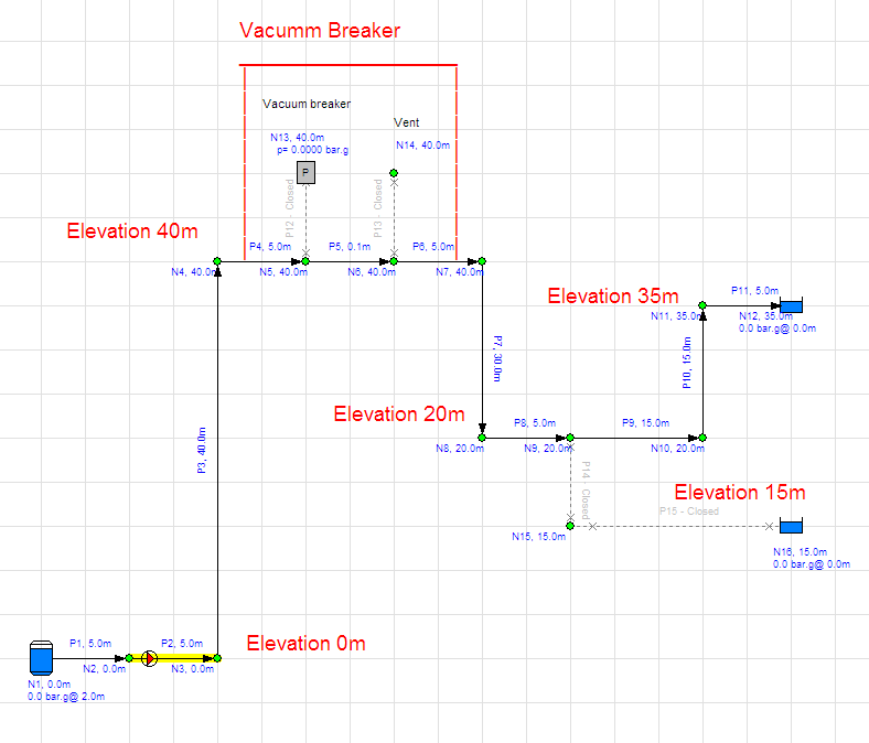
Consider the following system where a pump moves fluid from a low elevation point (0m), up and over a higher elevation point (40m), and on to some discharge location at an elevation point (35m) between the low and high point. The model shows a vaccum breaker arrangement BUT it is not operating (the pipes to the End Pressure and the Demand In-Flow that represent the vacuum breaker have been closed).

i.e. for all intents and purposes this is just a regular system (without the vaccum breaker)


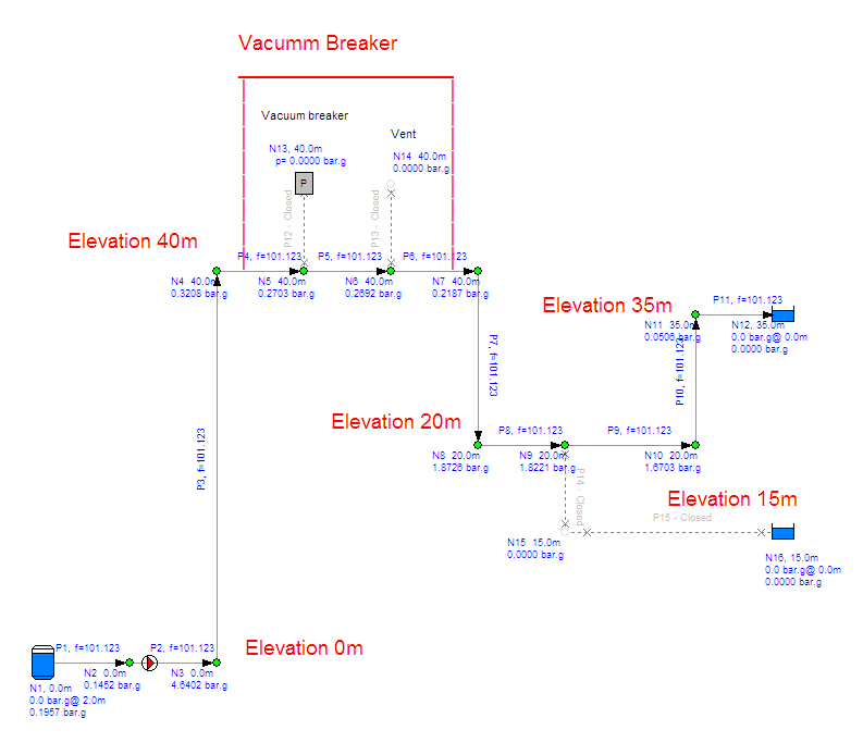
When solved, the system gives the results as shown in the following diagram, where you can see the pressure at node 4 is about 0.218 bar.g (still above the fluid vapour pressure) and there are no specific issues with low pressures in the model.



Example System 2

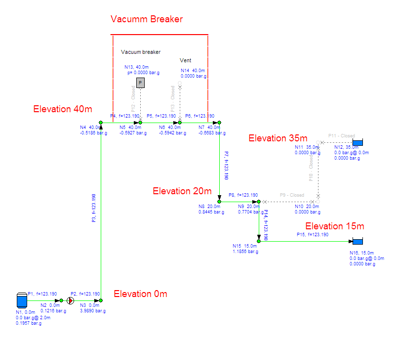
Consider the same system but now where pipes 9, 10, & 11 have been closed and pipes 14 and 15 have been opened, to allow flow to a lower discharge point.


When solved, the Pipe Flow Expert software shows that now the pressure at the high elevation points is below 0 bar.g. For example, the pressure at node 7 is now -0.66 bar.g.
Example System 3

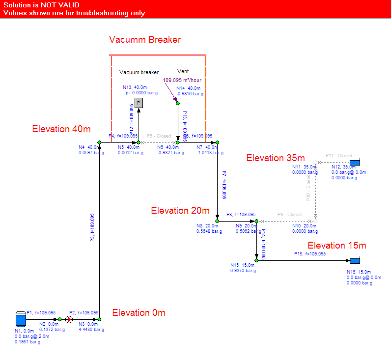
When unwanted vacuum conditions occur at the higher elevation points it is possible that a vacuum breaker may be introduced in to the system. In Pipe Flow Expert the vaccum breaker can be modelled by using an End Pressure and a Demand In-Flow as is shown in the following diagram. Essentially the system is split in to two separate systems. You can solve the model to find the flow rate in the first system and then this flow rate can be set as the Demand In-Flow at the start of the second system (the vent point).


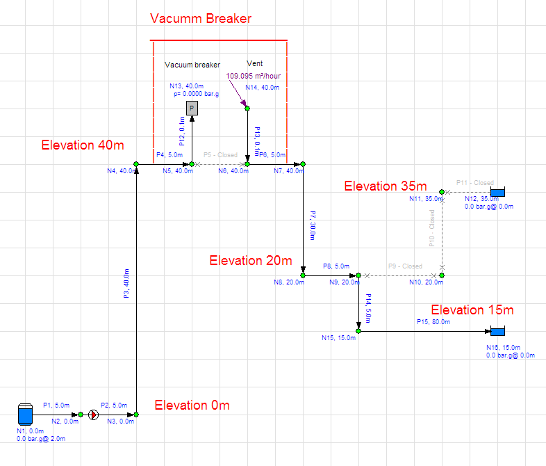
When solved, the Pipe Flow Expert software now warns that the solution is NOT VALID because a pressure has occured which is less than absolute zero (0 bar.a or -1 bar.g), however it permits the user to look at the calculated results in order to allow diagnosis of issues within the system. From the diagram below you can see that the pressure at node 7 is -1.04 bar.g.

This issue occurs because we have introduced the vacuum breaker which means the pressure at node 5 is now 0 bar.g and we have calculated the flow rate that occurs to this point (with 0 bar.g pressure there) and then we have set the same flow rate as the Demand In-Flow at node 14, BUT the Pipe Flow Expert software has calculated that the pressure required at node 14 to produce this flow rate would need to be a very low (-1.04 bar.g - which is impossible).


In the Real World

In the real world the above results could never occur because now that the vacuum breaker has been introduced in to the system the pipe going down from node 14 would no longer be fully charged and fluid would free fall down the pipe to some point where the fluid fills the pipe back to its fully charged operating condition.

The elevation at which this occurs will be the point where the flow rate down from that point on can be achieved with a fully charged pipe and a pressure of 0 bar.g at that point (the vent condition). The previous impossible results showed a pressure of -1.04 bar.g at node 14 which means we need to lose at least 10m of water head pressure to get to the 0 bar.g condition.

i.e. this means we can move at least 10m down the pipe (to lose 10m of head pressure with some air in the pipe occuring down to this point)

In addition if extra pressure has not been lost to friction with the free fall flow down the pipe (we still have 0 bar.g pressure at some point farther down the pipe) then it is likley that the pipe will become fully charged at a point more than 10m down from node 14.


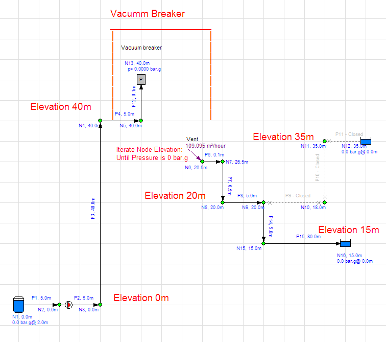
With some iteration, changing the elevation of node 6 and adjusting the other properties of pipe 7 to match, it is possible to find a solution where the Demand In-Flow set at 109.095 m^3/hour to match the flow rate produced in the first system, occurs with a pressure of approximately 0 bar.g at node 6. This is the elevation that the pipe would become full of fluid and fully charged again and it occurs at an elevation of about 26.5m as shown in the following results.


Summary

This above analysis makes some important assumptions about the flow that occurs in the model which are different than how flow will actually occur in the real world, however this approach will allow the engineer to obtain an approximate solution to the flows and pressures in their system where it contains a vacuum breaker.

In the real world, additonal head loss caused by two-phase flow between the vacuum breaker and the elevation at which the down pipe becomes fully charged and filled with fluid will occur, and this is neglected and not accounted for in the model above. If a more accurate solution is required then the engineer will need to find other software that can calculate for systems with two-phase flow (the Pipe Flow Expert software does not calculate for two-phase flow).

Also, the capacity of the vacuum breaker can affect the value of the vacuum that is obtained and this can affect the pressure and flows in the model.

The above information is provided as a suggested method to allow an engineer to produce a piping model that approximates the results for a system that contains a vacuum breaker, however it is up to the engineer to determine the suitability of applying such an approach to their model and to take account of the assumptions that are made with this approach and to assess and decide whether the results of such a model are accurate enough for the purpose that they will be used.